
Measurement Result [
 ]
]
Since measurement uncertainties indicate the quality of an experiment, no measurement result is complete without it. Next, the different ways of denoting the measurement result are shown followed by the rules on the number of significant figures that need to be shown.
Notation of measurement results []
A complete measurement result always shows the best estimation as well as the uncertainty. The most common way to denote this is: $$\text{Measurement result} = \text{best estimation} \pm \text{uncertainty}.\tag{5}$$ Der Bestwert ist meist der Mittelwert , und die Messunsicherheit die Standardabweichung σ. The best estimation is most often the mean value, x, and the uncertainty the standard deviation, σ.
The rounding of the best estimation goes in accordance with the digits of the uncertainty. The best estimation gets as many decimal places as the uncertainty has. For instance, suppose the following current is measured: I = 0.227 459 A with an uncertainty uI = 0.0050 A, see Fig. 4. The uncertainty has four decimal places, hence, the best estimation is rounded to four decimal places: $$I=(0.2275 \pm 0.0050)\text{ A}.\tag{6}$$
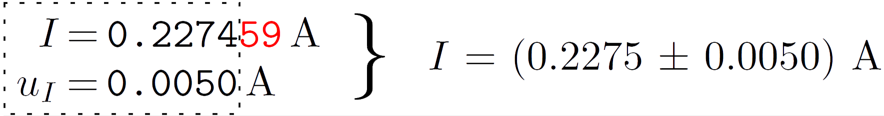
Figure 4: The best estimation of the current gets rounded according to the uncertainty of the current, i.e., four decimal places.
Another way to denote the uncertainty is by placing it in parentheses. This is best illustrated using the example from before. With the parentheses notation, this becomes: $$I=0.2275(50)\text{ A}.\tag{7}$$ This notation is slightly less intuitive for students. The DIN favors this notation for the industry since it sets itself apart from tolerance that has the same notation as (6). Tolerance indicates the maximum deviation between measurements and a reference value that is allowed in e.g., production processes.
The uncertainty is an indication of the precision of a measurement result and, hence, an indication of the quality of the experiment. The uncertainty spans an ⓘ uncertainty intervaluncertainty interval: The range of values spanned by the mean and the uncertainty. around the best estimation. The uncertainty interval ranges from: $$\text{uncertainty interval} = [\bar{x}-\sigma ; \bar{x}+\sigma].\tag{8}$$ The uncertainty interval can be seen as the range of values in which the measurand is to be expected (with a certain degree of confidence).
Again looking back on the measurement data of the falling distance of a ruler, see Fig. 5a, this measurement result can be represented graphically. The standard way to plot this is, is by using uncertainty bars (sometimes referred to as errorbars) as shown in Fig. 5b. Note that in this case, the uncertainty is shown for the variable on thex-axis, for uncertainties on the y-axis, the uncertainty bars are vertical.
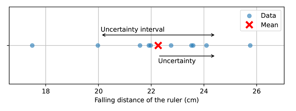
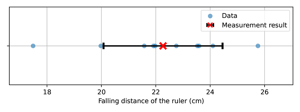
Figure 5: Measurement data of the falling distance of a ruler, like in Fig. 1 now with the complete measurement result.
Number of significant figures []
In the example from before, the uncertainty of the current was given in two ⓘ significant figuressignificant figures: The number of digits after the leading zeros.. The number of significant figures is the number of digits without counting the leading zeros, see Tab. 3.
Table 3: The number of significant figures in blue for given quantities.
| Quantity | significant figures |
|---|---|
| \(l= \textcolor{blue}{17.2}\text{ cm}\) | 3 |
| \(t = \textcolor{blue}{10.02}\text{ s}\) | 4 |
| \(V = 0.0\textcolor{blue}{250}\text{ L} = \textcolor{blue}{25.0}\text{ mL}\) | 3 |
| \(\lambda = \textcolor{blue}{640.0}\text{ nm} = \textcolor{blue}{6.400}\cdot 10^{-7}\text{ m}\) | 4 |
| \(d = 0.000\,0\textcolor{blue}{10}\text{ m} = \textcolor{blue}{10}\cdot 10^{-6}\text{ m} = 0.0\textcolor{blue}{10}\text{ mm}\) | 2 |
The number of significant figures of the uncertainty determines the number of significant figures of the best estimation, which is rounded in accordance with the uncertainty, see Fig. 4. It should be noted that, the number of significant figures of the best estimation is always larger or equal to the number of significant figures of the uncertainty. There exist three rules for the number of significant figures of the uncertainty:
- The uncertainty is written using one significant figure.
Examples:
u = 3.581 cm = 4 cm
u = 149 m = 1 · 102 m = 0.1 km
u = 0.005 01 A = 0.005 A = 5 mA
u = 0.029 48 L = 0.003 L - The uncertainty is written using two significant figures.
Examples:
u = 3.581 cm = 3.6 cm
u = 149 m = 1.5 · 102 m = 0.15 km
u = 0.005 01 A = 0.0050 A = 50 mA
u = 0.029 48 L = 0.0029 L - The uncertainty is written using one significant figure unless the first significant figure is a 1 or a 2, in which case two significant figures are indicated.
Examples:
u = 3.581 cm = 4 cm
u = 149 m = 1,5 · 102 m = 0,15 km
u = 0.005 01 A = 0.005 A = 5 mA
u = 0.029 48 L = 0.0029 L
The GUM [siehe 1] does not prefer a specific rule for the number of significant figures of the uncertainty (although they specify to use a maximum of two digits).
For the rounding of the uncertainty, there are two options: normal rounding (as was done above) or rounding up. Always rounding up (e.g., 0.005 01 A = 0.0051 A or even 0.005 01 A = 0.006 A) is a very conservative procedure that can lead to overestimations of the uncertainty. The GUM is somewhat ambivalent here but seems to prefer normal rounding. They do state that it is sometimes appropriate to round uncertainties up using common sense. This would mean to round u = 0.029 48 up to 0.030 L but to round u = 0.005 01 A down to 0.0050 A.
Students' ideas about the measurement result []
When asked how one should report a measurement result, many students (even at the university level) indicate that the mean value should be reported [2]. However, for a complete measurement result, this should be complemented by the uncertainty. To prompt students to think about this, one could ask them how their measurement result reflects the quality of their experiment.
Literature
- Joint Committee for Guides in Metrology. (2008). Evaluation of measurement – guide to the expression of uncertainty in measurement (JCGM 100:2008). JCGM. https://www.bipm.org/utils/common/documents/jcgm/JCGM_100_2008_E.pdf
- Leach, J., Millar, R., Ryder, J., Séré, M.-G., Hammelev, D., Niedderer, H., & Tselfes, V. (1998). Survey 2: Students' images of science as they relate to labwork learning. Working paper 4, labwork in science education project (Project PL 95-2005; p. 86). Centre for Studies in Science and Mathematics Education. https://essl.leeds.ac.uk/download/downloads/id/613/labwork_in_science_education_working_paper_4.pdf