
Type A [

 ]
]
In the previous step, all the basic concepts and terminology were covered. This step is concerned with the quantification of the uncertainty. This is done for repeated measurements, single measurements, and graphical analysis. After that, some rules for uncertainty propagation and the relative uncertainty are covered. Each part starts with the basics followed by didactical considerations.
When measurements are subject to variability, one should take repeated measurements to determine the measurement result (see Repeated Measurements). The uncertainty in these instances can be determined by statistical means. This type of uncertainty evaluation is called a ⓘ type Atype A: Evaluation of the uncertainty using statistics. uncertainty evaluation.
Reduction of complexity []
The standard deviation and the standard deviation of the mean (see Uncertainty) are the most common quantifications of the uncertainty in scientific practice. Often, students experience difficulties in the process of calculating and interpreting these [1–3]. To aid them, one could to automate the process of calculating the uncertainty, however, it has been found that students consequently lose a feeling for the credibility of the outcome [3].
Alternatively, one could graphically represent the measurements. This visualizes the variability of the measurements, which reduces the cognitive load on the students [4, 5]. However, this approach lacks a numerical quantification of the uncertainty, something favored by researchers, and something that would also be required for schools [1, 3].
Alternative quantifications []
Another option is to make use of other quantifications that are easier to calculate and conceptually understand. Next, four alternative quantifications will be defined. Research has shown that, when comparing these quantifications with the standard deviation, increasing mathematical complexity also increases the statistical quality [6].
The most simple quantification is the maximum deviation. To calculate this, one sorts all measurements from smallest (x1) to largest (xN) and calculates the mean value (x). The biggest difference between the mean value and the smallest or largest value of the series is the uncertainty: $$u_\text{max} = \max \big( \bar{x} - x_1, x_N - \bar{x} \big).\tag{9}$$ This measure is graphically shown in Fig. 6. The advantage of this quantification is its mathematical simplicity. Its disadvantage is that it is a big overestimation of the uncertainty (in comparison to the standard deviation) that is highly sensitive to outliers.
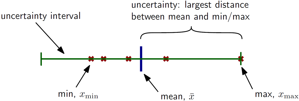
Figure 6: Graphical depiction of how the maximum deviation is calculated. The red crosses are the individual measurements, the blue bar indicates the mean value, and the uncertainty is the largest distance between the mean and either the min or max value of the data set. The green bar indicates the complete uncertainty interval around the mean value.
To compensate for outliers, this procedure can be adapted to exclude the smallest (x1) and largest (xN) value of the series and repeat the procedure for the remaining measurements. This is called the exclude extremes quantification: $$u_\text{excl.extr.} = \max \big( \bar{x} - x_2, x_{N-1} - \bar{x} \big).\tag{10}$$ This quantification is almost as simple as the maximum deviation, but is less sensitive for outliers. However, with an increasing number of repeated measurements, this quantification becomes equally sensitive for outliers.
For larger sample sizes, one could decide to repeat the procedure for the central half of the measurements, this is called the middle 50% measure. To do so, one starts excluding pairs of extreme values one by one until the remaining number of measurements would be less than half the total number of measurements. For instance, for 4–7 measurements, one pair of extremes is excluded, for 8–11 measurements two pairs are excluded, etc. In the form of an equation, this can be written as: $$u_\text{mid.50%} = \max \big( \bar{x} - x_{1 + N/4}, x_{N - N/4} - \bar{x} \big).\tag{11}$$ The downside for this measure is that it might feel unsatisfying for students. They might wonder why repeated measurements were taken at all when half their dataset is disregarded.
The last alternative is the mean absolute deviation (MAD). This is the average of all individual measurements' deviations from the mean: $$u_\text{MAD} = \frac{1}{N}\sum_{i=1}^N |x_i-\bar{x}|.\tag{12}$$ Since the calculation of the MAD involves the calculation of a mean value, it is conceptually easy to understand. This uncertainty gives a value that is systematically lower than the standard deviation.
Further reading []
For further information on the different uncertainty quantifications and some examples, see [7].
For some ideas for experiments where the analysis of the measurement uncertainty is a necessity for drawing a correct conclusion see: [8–14].
Literature
- Deardorff, D. L. (2001). Introductory Physics Students' Treatment of Measurement Uncertainty [Doctoral Thesis, North Carolina State University]. https://projects.ncsu.edu/PER//Articles/DeardorffDissertation.pdf
- Séré, M., Journeaux, R., & Larcher, C. (1993). Learning the statistical analysis of measurement errors. International Journal of Science Education, 15(4), 427–438. https://doi.org/10.1080/0950069930150406
- Zangl, H., & Hoermaier, K. (2017). Educational aspects of uncertainty calculation with software tools. Measurement, 101, 257–264. https://doi.org/10.1016/j.measurement.2015.11.005
- Kramer, R. S. S., Telfer, C. G. R., & Towler, A. (2017). Visual Comparison of Two Data Sets: Do People Use the Means and the Variability? Journal of Numerical Cognition, 3(1), 97–111. https://doi.org/10.5964/jnc.v3i1.100
- Susac, A., Bubic, A., Martinjak, P., Planinic, M., & Palmovic, M. (2017). Graphical representations of data improve student understanding of measurement and uncertainty: An eye-tracking study. Physical Review Physics Education Research, 13(2), 020125. https://doi.org/10.1103/PhysRevPhysEducRes.13.020125
- Kok, K., & Priemer, B. (2022). Comparing Different Uncertainty Measures to Quantify Measurement Uncertainties in High School Science Experiments. International Journal of Physics and Chemistry Education, 14(1), 1–9. https://doi.org/10.48550/arXiv.2205.04102
- Kok, K., & Priemer, B. (2023a). Messunsicherheiten quantifizieren: Welche Maße gibt es dafür? MNU Journal, 76(4), 330–333. https://doi.org/10.18452/27043
- Kok, K., Boczianowski, F., & Priemer, B. (2020). Messdaten im Physikunterricht auswerten – wann sind Messunsicherheiten wichtig? MNU Journal, 73(4), 292–295. https://doi.org/10.18452/27175
- Boczianowski, F., & Kok, K. (2020). Modelle empirisch prüfen—Frequenzmessung an stehenden akustischen Wellen mit dem Smartphone. MNU Journal, 73(4), 295–299.
- Kok, K., & Boczianowski, F. (2021). Acoustic Standing Waves: A Battle Between Models. The Physics Teacher, 59(3), 181–184. https://doi.org/10.1119/10.0003659
- Kok, K., & Priemer, B. (2023b). Using measurement uncertainties to detect incomplete assumptions about theory in an experiment with rolling marbles. Physics Education, 58(3), 035007. https://doi.org/10.1088/1361-6552/acb87b
- Musold, W., & Kok, K. (2025). Wie lang ist die Banane? — Über die Relevanz, eine Messgröße zu definieren. In B. Priemer & K. Kok (Hrs.), Messunsicherheiten im Physikunterricht (1. Aufl., S. 165–169). Berlin Universities Publishing. https://doi.org/10.14279/depositonce-21608
- Nagel, C. (2021). Messunsicherheiten im Schullaltag—Eine Kurzanleitung für Interessierte. Plus Lucis, 4, 12–13.
- Wagner, S., Maut, C., & Priemer, B. (2021). Thermal expansion of water in the science lab—Advantages and disadvantages of different experimental setups. Physics Education, 56(3), 035022. https://doi.org/10.1088/1361-6552/abeac4