
Graphs [ ]
]
Sometimes, determining a quantity is done, not by repeating measurements, but by looking at the dependence between two other variables. In this case, the data is usually evaluated by using a graph and a trendline or fit function.
Determining the uncertainty of a fit function [ ]
]
Suppose one wants to determine the resistance of a resistor R. To do so, one can vary and measure the electric potential U and measure the resulting current I. The different measurements can be plotted in a (U,I)-diagram, see Fig. 8a. A linear trendline (fit) of the shape y = ax + b can be fitted to the data, see Fig. 8b. Most computer programs (Excel, Qti-Plot, Google Sheets, ...) use the method of least squares. The result of this procedure gives the slope a and (when desired) the y-axis offset b.
Using Ohm's law (I=U/R), one can calculate the resistance using the slope a which is equal to 1/R. In this case, the resistance is calculated to be 96.3 Ω.
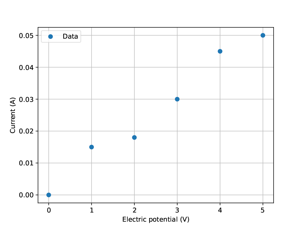
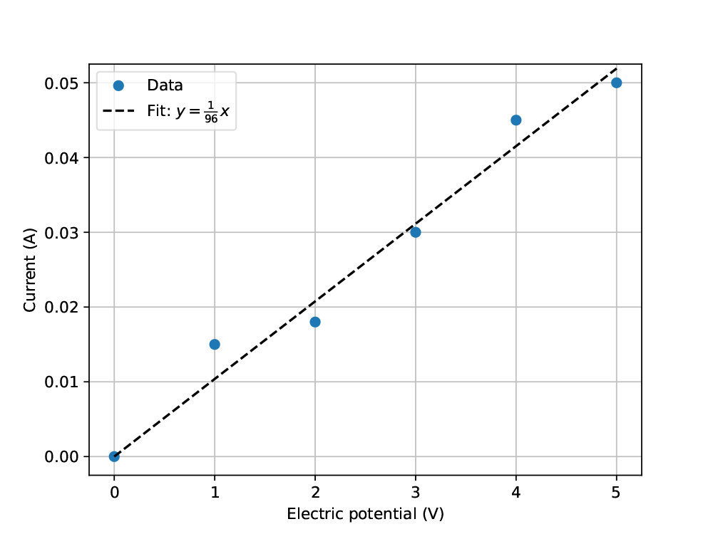
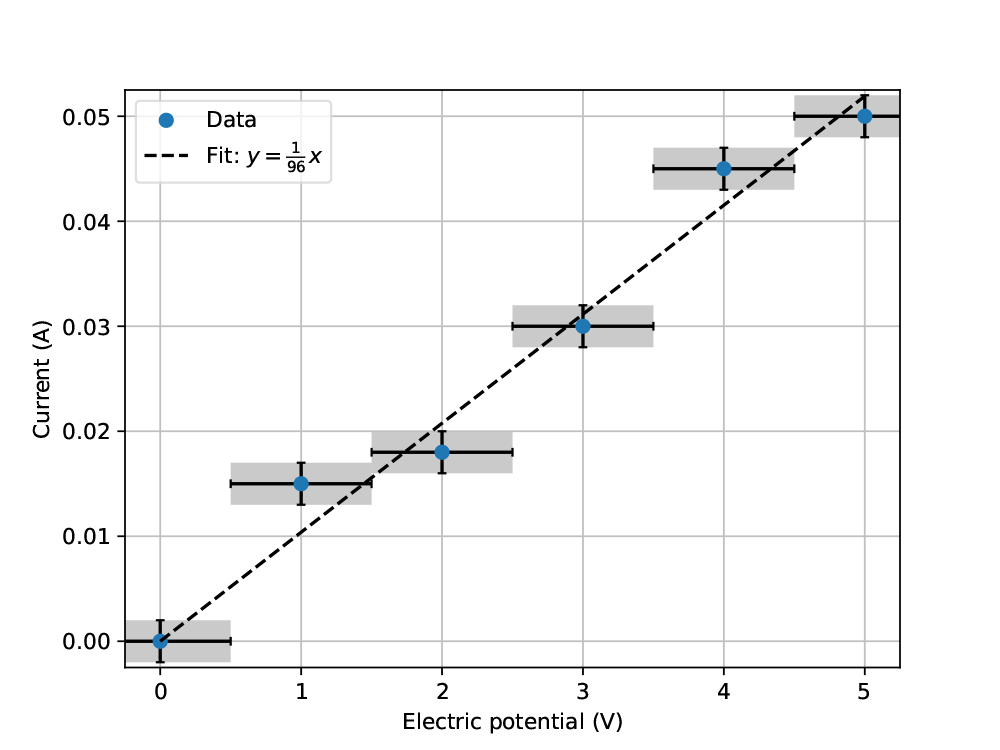
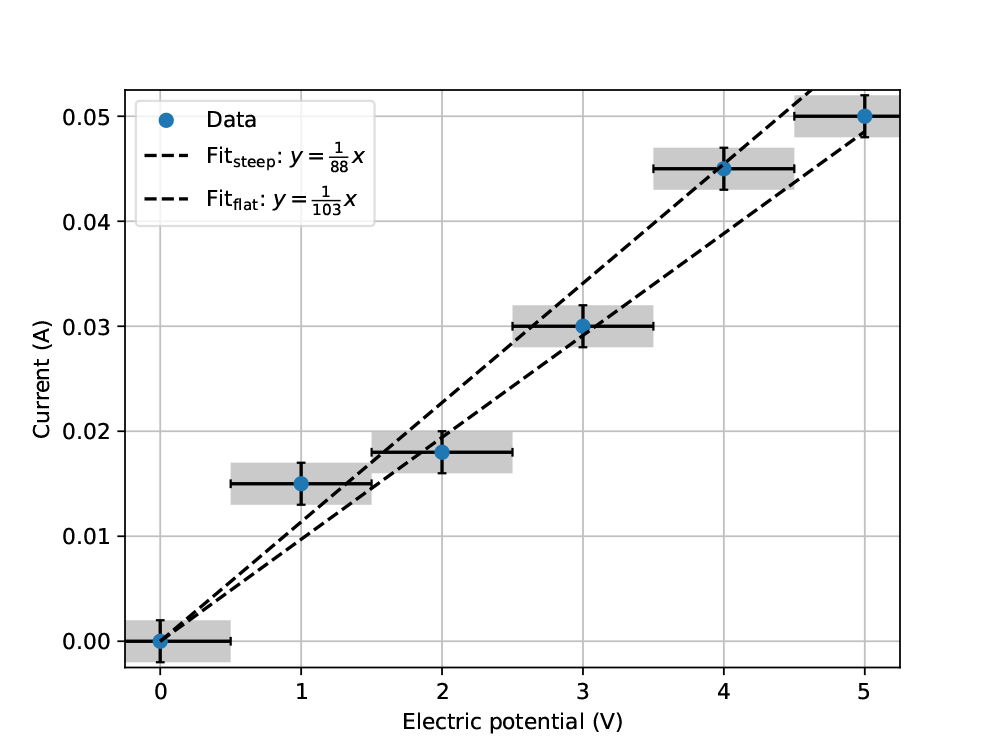
Figure 8: Different plots of measurement data from the electric potential over, and the current going through a resistor.
However, this graph does not show whether the fit truly "fits" the data. This can only be determined by looking at the measurement uncertainty, see Fig. 8c. This figure shows that the fit goes through all the uncertainty boxes (the gray shaded areas that span the uncertainty intervalls in the potential and current) and thus is a good fit to the data. At this point, one could say that the resistance of the resistor has a best estimation of R = 96.3 Ω.
To determine the uncertainty of the fit function, one can refer back to the method of least squares to calculate this. This would yield uR = 3.7 Ω, so R = (96.3 ± 3.7) Ω. The exact procedure, however, goes beyond the scope of this unit.
Alternative graphical uncertainty determination [ ]
]
There is a more simplified, graphical, method to determine the uncertainty. This is done by drawing the steepest and the flattest fit function that still goes through all the uncertainty boxes and determine these slopes, see Fig. 8d. This yields a slope with resistances of R = 88 Ω and R = 103 Ω. Using the same process that was used for the maximum deviation (see Eq. (9))), this yields an uncertainty of uR = 8 Ω, such that R = (96 ± 8) Ω.
In the latter example, this method clearly overestimates the uncertainty. In other instances, usually when the uncertainties per data point are small, this method will result in too small uncertainties. Sometimes, the method appears to not work at all since there exists no line that goes through all uncertainty boxes. In these cases, it is important to remember that even the method of least squares will not go through all uncertainty boxes but still give a result. One should draw a line that goes through the uncertainty boxes as well as possible. The steepest and flattest slopes should be drawn in the same manner.
The big advantage of this method is that no complex statistical methods are required and it can even be done using paper and pencil.
Fitting a model [ ]
]
A practical example of a low-cost high school experiment where two model functions are compared with data can be found here: [1]. The two models correspond to two functions and in the experiment and there is a check whether the data fits one of these functions. This fit would indicate which of the two models describes the data best.
Literature
- Kok, K., & Boczianowski, F. (2021). Acoustic Standing Waves: A Battle Between Models. The Physics Teacher, 59(3), 181–184. https://doi.org/10.1119/10.0003659